Two-Body Relativistic Kinematics Calculation
Consider the two-body reaction m 1 ( m 2 , m 3 ) m 4 m_1(m_2, m_3)m_4 m 1 ( m 2 , m 3 ) m 4
We use units in which c = 1 c=1 c = 1
( 1 − 1 − 1 − 1 ) \mqty(
\dmat{
1, -1, -1, -1
}
) 1 − 1 − 1 − 1 Let β G \beta_G β G
( γ G − β G γ G − β G γ G γ G ) ( E 1 ( l a b ) p 1 ( l a b ) ) \mqty(
\gamma_G & - \beta_G \gamma_G \\
- \beta_G \gamma_G & \gamma_G
)
\mqty(
E_1^\mathrm{(lab)} \\
p_1^\mathrm{(lab)}
) ( γ G − β G γ G − β G γ G γ G ) ( E 1 ( lab ) p 1 ( lab ) ) ( γ G − β G γ G − β G γ G γ G ) ( E 2 ( l a b ) p 2 ( l a b ) ) \mqty(
\gamma_G & - \beta_G \gamma_G \\
- \beta_G \gamma_G & \gamma_G
)
\mqty(
E_2^\mathrm{(lab)} \\
p_2^\mathrm{(lab)}
) ( γ G − β G γ G − β G γ G γ G ) ( E 2 ( lab ) p 2 ( lab ) ) The velocity β \beta β γ \gamma γ
γ 2 − β 2 γ 2 = 1 \gamma^2
- \beta^2\gamma^2
= 1 γ 2 − β 2 γ 2 = 1 We can therefore introduce the rapidity χ \chi χ
cosh χ = γ , sinh χ = β γ . \cosh \chi = \gamma,\quad
\sinh \chi = \beta \gamma. cosh χ = γ , sinh χ = β γ . and write the boost matrix as
( cosh χ − sinh χ − sinh χ cosh χ ) \mqty(
\cosh \chi & - \sinh \chi \\
- \sinh \chi & \cosh \chi
) ( cosh χ − sinh χ − sinh χ cosh χ ) This form is used in the SkiSickness explanation .
The total momentum vanishes in the CM frame, p 1 ( C M ) + p 2 ( C M ) = 0 p_1^\mathrm{(CM)} + p_2^\mathrm{(CM)} = 0 p 1 ( CM ) + p 2 ( CM ) = 0
β G = p 1 ( l a b ) + p 2 ( l a b ) E 1 ( l a b ) + E 2 ( l a b ) , γ G = 1 1 − β G 2 . \beta_G
= \frac{
p_1^\mathrm{(lab)} + p_2^\mathrm{(lab)}
}{
E_1^\mathrm{(lab)} + E_2^\mathrm{(lab)}
}, \quad
\gamma_G
= \frac{1}{\sqrt{1-\beta_G^2}} . β G = E 1 ( lab ) + E 2 ( lab ) p 1 ( lab ) + p 2 ( lab ) , γ G = 1 − β G 2 1 . The Mandelstam variable s s s
s = ( p 1 + p 2 ) 2 = ( E 1 + E 2 ) 2 − ( p 1 + p 2 ) 2 s
= (p_1 + p_2)^2
= (E_1 + E_2)^2 - (p_1 + p_2)^2 s = ( p 1 + p 2 ) 2 = ( E 1 + E 2 ) 2 − ( p 1 + p 2 ) 2 If target particle 1 is at rest and incident particle 2 has kinetic energy T T T
s = ( m 1 + m 2 + T ) 2 − p 2 ( l a b ) 2 = ( m 1 + m 2 + T ) 2 − ( ( m 2 + T ) 2 − m 2 2 ) = ( m 1 + m 2 ) 2 + 2 m 1 T s
= (m_1 + m_2 + T)^2 - p_2^{\mathrm{(lab)}2}
= (m_1 + m_2 + T)^2 - \qty( (m_2 + T)^2 - m_2^2 )
= (m_1 + m_2)^2 + 2m_1T s = ( m 1 + m 2 + T ) 2 − p 2 ( lab ) 2 = ( m 1 + m 2 + T ) 2 − ( ( m 2 + T ) 2 − m 2 2 ) = ( m 1 + m 2 ) 2 + 2 m 1 T Since s s s
s = ( E 1 ( C M ) + E 2 ( C M ) ) 2 − ( p 1 ( C M ) + p 2 ( C M ) ) 2 = ( m 1 2 + p 1 ( C M ) 2 + m 2 2 + p 1 ( C M ) 2 ) 2 s
= \qty( E_1^\mathrm{(CM)} + E_2^\mathrm{(CM)} )^2
- \qty(p_1^\mathrm{(CM)} + p_2^\mathrm{(CM)})^2
= \qty(
\sqrt{ m_1^2 + p_1^{\mathrm{(CM)}2} }
+ \sqrt{ m_2^2 + p_1^{\mathrm{(CM)}2} }
)^2 s = ( E 1 ( CM ) + E 2 ( CM ) ) 2 − ( p 1 ( CM ) + p 2 ( CM ) ) 2 = ( m 1 2 + p 1 ( CM ) 2 + m 2 2 + p 1 ( CM ) 2 ) 2 Rearranging gives
2 m 1 2 + p 1 ( C M ) 2 m 2 2 + p 1 ( C M ) 2 = s − m 1 2 − m 2 2 − 2 p 1 ( C M ) 2 2 \sqrt{ m_1^2 + p_1^{\mathrm{(CM)}2} } \sqrt{ m_2^2 + p_1^{\mathrm{(CM)}2} }
= s - m_1^2 - m_2^2 - 2 p_1^{\mathrm{(CM)}2} 2 m 1 2 + p 1 ( CM ) 2 m 2 2 + p 1 ( CM ) 2 = s − m 1 2 − m 2 2 − 2 p 1 ( CM ) 2 4 m 1 2 m 2 2 + 4 ( m 1 2 + m 2 2 ) p 1 ( C M ) 2 + 4 p 1 ( C M ) 4 = ( m 1 2 + m 2 2 ) 2 + 4 ( m 1 2 + m 2 2 ) p 1 ( C M ) 2 + 4 p 1 ( C M ) 4 + s 2 − 2 s ( m 1 2 + m 2 2 + 2 p 1 ( C M ) 2 ) 4 m_1^2m_2^2
+ 4 (m_1^2 + m_2^2) p_1^{\mathrm{(CM)}2}
+ 4 p_1^{\mathrm{(CM)}4}
= (m_1^2 + m_2^2)^2
+ 4 (m_1^2 + m_2^2) p_1^{\mathrm{(CM)}2}
+ 4 p_1^{\mathrm{(CM)}4}
+ s^2
- 2 s \qty( m_1^2 + m_2^2 + 2 p_1^{\mathrm{(CM)}2}) 4 m 1 2 m 2 2 + 4 ( m 1 2 + m 2 2 ) p 1 ( CM ) 2 + 4 p 1 ( CM ) 4 = ( m 1 2 + m 2 2 ) 2 + 4 ( m 1 2 + m 2 2 ) p 1 ( CM ) 2 + 4 p 1 ( CM ) 4 + s 2 − 2 s ( m 1 2 + m 2 2 + 2 p 1 ( CM ) 2 ) 4 m 1 2 m 2 2 = ( m 1 2 + m 2 2 ) 2 + s 2 − 2 s ( m 1 2 + m 2 2 + 2 p 1 ( C M ) 2 ) 4 m_1^2m_2^2
= (m_1^2 + m_2^2)^2
+ s^2
- 2 s \qty( m_1^2 + m_2^2 + 2 p_1^{\mathrm{(CM)}2}) 4 m 1 2 m 2 2 = ( m 1 2 + m 2 2 ) 2 + s 2 − 2 s ( m 1 2 + m 2 2 + 2 p 1 ( CM ) 2 ) m 1 4 + m 2 4 − 2 m 1 2 m 2 2 + s 2 − 2 s ( m 1 2 + m 2 2 + 2 p 1 ( C M ) 2 ) = 0 m_1^4 + m_2^4 - 2m_1^2m_2^2
+ s^2
- 2 s \qty( m_1^2 + m_2^2 + 2 p_1^{\mathrm{(CM)}2})
= 0 m 1 4 + m 2 4 − 2 m 1 2 m 2 2 + s 2 − 2 s ( m 1 2 + m 2 2 + 2 p 1 ( CM ) 2 ) = 0 4 s p 1 ( C M ) 2 + 2 s ( m 1 2 + m 2 2 ) − s 2 − ( m 1 2 − m 2 2 ) 2 = 0 4 s p_1^{\mathrm{(CM)}2}
+ 2 s (m_1^2 + m_2^2)
- s^2
- (m_1^2 - m_2^2)^2
= 0 4 s p 1 ( CM ) 2 + 2 s ( m 1 2 + m 2 2 ) − s 2 − ( m 1 2 − m 2 2 ) 2 = 0 p 1 ( C M ) 2 = ( m 1 2 − m 2 2 ) 2 + s 2 − 2 s ( m 1 2 + m 2 2 ) 4 s = { s − ( m 1 2 + m 2 2 ) } 2 − 4 m 1 2 m 2 2 4 s \begin{align*}
p_1^{\mathrm{(CM)}2}
&= \frac{
(m_1^2 - m_2^2)^2
+ s^2
-2s (m_1^2 + m_2^2)
}{
4s
}\\
&= \frac{
\qty{
s
- \qty(m_1^2 + m_2^2)
}^2
- 4 m_1^2 m_2^2
}{
4s
}
\end{align*} p 1 ( CM ) 2 = 4 s ( m 1 2 − m 2 2 ) 2 + s 2 − 2 s ( m 1 2 + m 2 2 ) = 4 s { s − ( m 1 2 + m 2 2 ) } 2 − 4 m 1 2 m 2 2 p 1 ( C M ) = { s − ( m 1 2 + m 2 2 ) } 2 − 4 m 1 2 m 2 2 4 s p_1^{\mathrm{(CM)}}
= \sqrt{
\frac{
\qty{
s
- \qty(m_1^2 + m_2^2)
}^2
- 4 m_1^2 m_2^2
}{
4s
}
} p 1 ( CM ) = 4 s { s − ( m 1 2 + m 2 2 ) } 2 − 4 m 1 2 m 2 2 E 1 ( C M ) = m 1 γ G = m 1 cosh χ = m 1 2 + p 1 ( C M ) 2 E_1^{\mathrm{(CM)}}
= m_1 \gamma_G
= m_1 \cosh \chi
= \sqrt{m_1^2 + p_1^{\mathrm{(CM)}2} } E 1 ( CM ) = m 1 γ G = m 1 cosh χ = m 1 2 + p 1 ( CM ) 2 p 1 ( C M ) = m 1 β G γ G = m 1 sinh χ = p 1 ( C M ) p_1^{\mathrm{(CM)}}
= m_1 \beta_G \gamma_G
= m_1 \sinh \chi
= p_1^{\mathrm{(CM)}} p 1 ( CM ) = m 1 β G γ G = m 1 sinh χ = p 1 ( CM ) we obtain
cosh χ = m 1 2 + p 1 ( C M ) 2 m 1 , sinh χ = p 1 ( C M ) m 1 . \cosh \chi
= \frac{\sqrt{m_1^2 + p_1^{\mathrm{(CM)}2}}}{m_1}, \quad
\sinh \chi
= \frac{p_1^{\mathrm{(CM)}}}{m_1}. cosh χ = m 1 m 1 2 + p 1 ( CM ) 2 , sinh χ = m 1 p 1 ( CM ) . Using sinh χ + cosh χ = exp χ \sinh \chi + \cosh \chi = \exp \chi sinh χ + cosh χ = exp χ
χ = ln ( p 1 ( C M ) + m 1 2 + p 1 ( C M ) 2 m 1 ) \chi
= \ln\qty(
\frac{
p_1^{\mathrm{(CM)}}
+ \sqrt{m_1^2 + p_1^{\mathrm{(CM)}2}}
}{m_1}
) χ = ln m 1 p 1 ( CM ) + m 1 2 + p 1 ( CM ) 2 Conservation of four-momentum gives the same value of s s s p 3 ( C M ) + p 4 ( C M ) = 0 p_3^{\mathrm{(CM)}} + p_4^{\mathrm{(CM)}} = 0 p 3 ( CM ) + p 4 ( CM ) = 0
s = ( E 3 ( C M ) + E 4 ( C M ) ) 2 = ( m 3 2 + p 3 ( C M ) 2 + m 4 2 + p 4 ( C M ) 2 ) 2 \begin{align*}
s
&= \qty(E_3^{\mathrm{(CM)}} + E_4^{\mathrm{(CM)}})^2 \\
&= \qty(
\sqrt{
m_3^2 + p_3^{\mathrm{(CM)}2}
}
+ \sqrt{
m_4^2 + p_4^{\mathrm{(CM)}2}
}
)^2
\end{align*} s = ( E 3 ( CM ) + E 4 ( CM ) ) 2 = ( m 3 2 + p 3 ( CM ) 2 + m 4 2 + p 4 ( CM ) 2 ) 2 Following the same steps as above, we obtain
p 3 ( C M ) = { s − ( m 3 2 + m 4 2 ) } 2 − 4 m 3 2 m 4 2 4 s p_3^{\mathrm{(CM)}}
= \sqrt{
\frac{
\qty{
s
- \qty(m_3^2 + m_4^2)
}^2
- 4 m_3^2 m_4^2
}{
4s
}
} p 3 ( CM ) = 4 s { s − ( m 3 2 + m 4 2 ) } 2 − 4 m 3 2 m 4 2 We can now calculate the CM energies of particles 3 and 4, E 3 ( C M ) E_3^{\mathrm{(CM)}} E 3 ( CM ) E 4 ( C M ) E_4^{\mathrm{(CM)}} E 4 ( CM )
E 3 ( C M ) 2 = m 3 2 + p 3 ( C M ) 2 = m 3 2 + { s − ( m 3 2 + m 4 2 ) } 2 − 4 m 3 2 m 4 2 4 s = { s + ( m 3 2 − m 4 2 ) } 2 4 s \begin{align*}
E_3^{\mathrm{(CM)}2}
&= m_3^2 + p_3^{\mathrm{(CM)}2}\\
&= m_3^2 + \frac{
\qty{s - \qty(m_3^2 + m_4^2)}^2- 4 m_3^2 m_4^2
}{4s}\\
&= \frac{
\qty{s + \qty(m_3^2 - m_4^2)}^2
}{
4s
}
\end{align*} E 3 ( CM ) 2 = m 3 2 + p 3 ( CM ) 2 = m 3 2 + 4 s { s − ( m 3 2 + m 4 2 ) } 2 − 4 m 3 2 m 4 2 = 4 s { s + ( m 3 2 − m 4 2 ) } 2 E 3 ( C M ) = s + ( m 3 2 − m 4 2 ) 2 s E_3^{\mathrm{(CM)}}
= \frac{
s + \qty(m_3^2 - m_4^2)
}{
2 \sqrt{s}
} E 3 ( CM ) = 2 s s + ( m 3 2 − m 4 2 ) Since E 3 ( C M ) + E 4 ( C M ) = s E_3^{\mathrm{(CM)}} + E_4^{\mathrm{(CM)}} = \sqrt{s} E 3 ( CM ) + E 4 ( CM ) = s
E 4 ( C M ) = s − ( m 3 2 − m 4 2 ) 2 s E_4^{\mathrm{(CM)}}
= \frac{
s - \qty(m_3^2 - m_4^2)
}{
2 \sqrt{s}
} E 4 ( CM ) = 2 s s − ( m 3 2 − m 4 2 ) In the CM frame, particles 3 and 4 have equal and opposite momenta.
Their four-momenta, written here using the component along particle 3's direction of motion, are
( E 3 ( C M ) p 3 ( C M ) ) , ( E 4 ( C M ) − p 3 ( C M ) ) . \mqty(
E_3^{\mathrm{(CM)}} \\
p_3^{\mathrm{(CM)}}
), \quad
\mqty(
E_4^{\mathrm{(CM)}} \\
- p_3^{\mathrm{(CM)}}
). ( E 3 ( CM ) p 3 ( CM ) ) , ( E 4 ( CM ) − p 3 ( CM ) ) . We apply the inverse Lorentz boost to return to the lab frame.
The boost acts on the energy and the momentum component along the beam axis:
( γ G β G γ G β G γ G γ G ) ( E 3 ( C M ) p 3 ( C M ) cos θ ( C M ) ) = ( γ G E 3 ( C M ) + β G γ G p 3 ( C M ) cos θ ( C M ) β G γ G E 3 ( C M ) + γ G p 3 ( C M ) cos θ ( C M ) ) = ( E 3 ( l a b ) p 3 ( l a b ) cos θ 3 ( l a b ) ) \mqty(
\gamma_G & \beta_G \gamma_G \\
\beta_G \gamma_G & \gamma_G
)
\mqty(
E_3^{\mathrm{(CM)}} \\
p_3^{\mathrm{(CM)}} \cos \theta^{\mathrm{(CM)}}
)
= \mqty(
\gamma_G E_3^{\mathrm{(CM)}} + \beta_G \gamma_G p_3^{\mathrm{(CM)}} \cos \theta^{\mathrm{(CM)}} \\
\beta_G \gamma_G E_3^{\mathrm{(CM)}} + \gamma_G p_3^{\mathrm{(CM)}} \cos \theta^{\mathrm{(CM)}}
)
= \mqty(
E_3^{\mathrm{(lab)}} \\
p_3^{\mathrm{(lab)}} \cos \theta_3^{\mathrm{(lab)}}
) ( γ G β G γ G β G γ G γ G ) ( E 3 ( CM ) p 3 ( CM ) cos θ ( CM ) ) = ( γ G E 3 ( CM ) + β G γ G p 3 ( CM ) cos θ ( CM ) β G γ G E 3 ( CM ) + γ G p 3 ( CM ) cos θ ( CM ) ) = ( E 3 ( lab ) p 3 ( lab ) cos θ 3 ( lab ) ) ( γ G β G γ G β G γ G γ G ) ( E 4 ( C M ) − p 3 ( C M ) cos θ 3 ( C M ) ) = ( γ G E 4 ( C M ) − β G γ G p 3 ( C M ) cos θ ( C M ) β G γ G E 4 ( C M ) − γ G p 3 ( C M ) cos θ ( C M ) ) = ( E 4 ( l a b ) p 4 ( l a b ) cos θ 4 ( l a b ) ) \mqty(
\gamma_G & \beta_G \gamma_G \\
\beta_G \gamma_G & \gamma_G
)
\mqty(
E_4^{\mathrm{(CM)}} \\
- p_3^{\mathrm{(CM)}} \cos \theta_3^{\mathrm{(CM)}}
)
= \mqty(
\gamma_G E_4^{\mathrm{(CM)}} - \beta_G \gamma_G p_3^{\mathrm{(CM)}} \cos \theta^{\mathrm{(CM)}} \\
\beta_G \gamma_G E_4^{\mathrm{(CM)}} - \gamma_G p_3^{\mathrm{(CM)}} \cos \theta^{\mathrm{(CM)}}
)
= \mqty(
E_4^{\mathrm{(lab)}} \\
p_4^{\mathrm{(lab)}} \cos \theta_4^{\mathrm{(lab)}}
) ( γ G β G γ G β G γ G γ G ) ( E 4 ( CM ) − p 3 ( CM ) cos θ 3 ( CM ) ) = ( γ G E 4 ( CM ) − β G γ G p 3 ( CM ) cos θ ( CM ) β G γ G E 4 ( CM ) − γ G p 3 ( CM ) cos θ ( CM ) ) = ( E 4 ( lab ) p 4 ( lab ) cos θ 4 ( lab ) ) The transverse momentum components are unchanged by the boost:
p 3 ( C M ) sin θ ( C M ) = p 3 ( l a b ) sin θ 3 ( l a b ) p 4 ( C M ) sin θ ( C M ) = p 4 ( l a b ) sin θ 4 ( l a b ) \begin{align*}
p_3^{\mathrm{(CM)}} \sin \theta^{\mathrm{(CM)}}
&= p_3^{\mathrm{(lab)}} \sin \theta_3^{\mathrm{(lab)}} \\
p_4^{\mathrm{(CM)}} \sin \theta^{\mathrm{(CM)}}
&= p_4^{\mathrm{(lab)}} \sin \theta_4^{\mathrm{(lab)}} \\
\end{align*} p 3 ( CM ) sin θ ( CM ) p 4 ( CM ) sin θ ( CM ) = p 3 ( lab ) sin θ 3 ( lab ) = p 4 ( lab ) sin θ 4 ( lab ) The kinetic energies in the lab frame are therefore
T 3 ( l a b ) = E 3 ( l a b ) − m 3 , T 4 ( l a b ) = E 4 ( l a b ) − m 4 . T_3^{\mathrm{(lab)}}
= E_3^{\mathrm{(lab)}} - m_3, \quad
T_4^{\mathrm{(lab)}}
= E_4^{\mathrm{(lab)}} - m_4. T 3 ( lab ) = E 3 ( lab ) − m 3 , T 4 ( lab ) = E 4 ( lab ) − m 4 . The squared momentum magnitudes in the lab frame are
p 3 ( l a b ) 2 = ( p 3 ( l a b ) sin θ 3 ( l a b ) ) 2 + ( p 3 ( l a b ) cos θ 3 ( l a b ) ) 2 , p 4 ( l a b ) 2 = ( p 4 ( l a b ) sin θ 4 ( l a b ) ) 2 + ( p 4 ( l a b ) cos θ 4 ( l a b ) ) 2 . \begin{align*}
p_3^{\mathrm{(lab)}2}
&= \qty(
p_3^{\mathrm{(lab)}} \sin \theta_3^{\mathrm{(lab)}}
)^2
+ \qty(
p_3^{\mathrm{(lab)}} \cos \theta_3^{\mathrm{(lab)}}
)^2 ,\\
p_4^{\mathrm{(lab)}2}
&= \qty(
p_4^{\mathrm{(lab)}} \sin \theta_4^{\mathrm{(lab)}}
)^2
+ \qty(
p_4^{\mathrm{(lab)}} \cos \theta_4^{\mathrm{(lab)}}
)^2 .
\end{align*} p 3 ( lab ) 2 p 4 ( lab ) 2 = ( p 3 ( lab ) sin θ 3 ( lab ) ) 2 + ( p 3 ( lab ) cos θ 3 ( lab ) ) 2 , = ( p 4 ( lab ) sin θ 4 ( lab ) ) 2 + ( p 4 ( lab ) cos θ 4 ( lab ) ) 2 . The lab-frame angles are given by
θ 3 ( l a b ) = arctan ( p 3 ( l a b ) sin θ 3 ( l a b ) p 3 ( l a b ) cos θ 3 ( l a b ) ) = arctan ( p 3 ( C M ) sin θ 3 ( C M ) β G γ G E 3 ( C M ) + γ G p 3 ( C M ) cos θ ( C M ) ) θ 4 ( l a b ) = arctan ( p 4 ( l a b ) sin θ 4 ( l a b ) p 4 ( l a b ) cos θ 4 ( l a b ) ) = arctan ( p 3 ( C M ) sin θ 3 ( C M ) β G γ G E 4 ( C M ) − γ G p 3 ( C M ) cos θ ( C M ) ) \begin{align*}
\theta_3^{\mathrm{(lab)}}
&= \arctan\qty(
\frac{
p_3^{\mathrm{(lab)}} \sin \theta_3^{\mathrm{(lab)}}
}{
p_3^{\mathrm{(lab)}} \cos \theta_3^{\mathrm{(lab)}}
}
)
= \arctan\qty(
\frac{
p_3^{\mathrm{(CM)}} \sin \theta_3^{\mathrm{(CM)}}
}{
\beta_G \gamma_G E_3^{\mathrm{(CM)}} + \gamma_G p_3^{\mathrm{(CM)}} \cos \theta^{\mathrm{(CM)}}
}
)
\\
\theta_4^{\mathrm{(lab)}}
&= \arctan\qty(
\frac{
p_4^{\mathrm{(lab)}} \sin \theta_4^{\mathrm{(lab)}}
}{
p_4^{\mathrm{(lab)}} \cos \theta_4^{\mathrm{(lab)}}
}
)
= \arctan\qty(
\frac{
p_3^{\mathrm{(CM)}} \sin \theta_3^{\mathrm{(CM)}}
}{
\beta_G \gamma_G E_4^{\mathrm{(CM)}} - \gamma_G p_3^{\mathrm{(CM)}} \cos \theta^{\mathrm{(CM)}}
}
)
\end{align*} θ 3 ( lab ) θ 4 ( lab ) = arctan ( p 3 ( lab ) cos θ 3 ( lab ) p 3 ( lab ) sin θ 3 ( lab ) ) = arctan ( β G γ G E 3 ( CM ) + γ G p 3 ( CM ) cos θ ( CM ) p 3 ( CM ) sin θ 3 ( CM ) ) = arctan ( p 4 ( lab ) cos θ 4 ( lab ) p 4 ( lab ) sin θ 4 ( lab ) ) = arctan ( β G γ G E 4 ( CM ) − γ G p 3 ( CM ) cos θ ( CM ) p 3 ( CM ) sin θ 3 ( CM ) ) tan θ 3 ( l a b ) = p 3 ( l a b ) sin θ 3 ( l a b ) p 3 ( l a b ) cos θ 3 ( l a b ) = p 3 ( C M ) sin θ 3 ( C M ) γ p 3 ( C M ) cos θ 3 ( C M ) + β γ E 3 ( C M ) \tan \theta_3^{\mathrm{(lab)}}
= \frac{
p_3^{\mathrm{(lab)}} \sin \theta_3^{\mathrm{(lab)}}
}{
p_3^{\mathrm{(lab)}} \cos \theta_3^{\mathrm{(lab)}}
}
= \frac{
p_3^{\mathrm{(CM)}} \sin \theta_3^{\mathrm{(CM)}}
}{
\gamma p_3^{\mathrm{(CM)}} \cos \theta_3^{\mathrm{(CM)}}
+ \beta \gamma E_3^{\mathrm{(CM)}}
} tan θ 3 ( lab ) = p 3 ( lab ) cos θ 3 ( lab ) p 3 ( lab ) sin θ 3 ( lab ) = γ p 3 ( CM ) cos θ 3 ( CM ) + β γ E 3 ( CM ) p 3 ( CM ) sin θ 3 ( CM ) γ tan θ 3 ( l a b ) cos θ 3 ( C M ) − sin θ 3 ( C M ) = − β γ E 3 ( C M ) tan θ 3 ( l a b ) p 3 ( C M ) \gamma \tan \theta_3^{\mathrm{(lab)}} \cos \theta_3^{\mathrm{(CM)}}
- \sin \theta_3^{\mathrm{(CM)}}
= - \frac{
\beta \gamma E_3^{\mathrm{(CM)}} \tan \theta_3^{\mathrm{(lab)}}
}{
p_3^{\mathrm{(CM)}}
} γ tan θ 3 ( lab ) cos θ 3 ( CM ) − sin θ 3 ( CM ) = − p 3 ( CM ) β γ E 3 ( CM ) tan θ 3 ( lab ) cos ( θ 3 ( C M ) + α ) = − β γ E 3 ( C M ) tan θ 3 ( l a b ) p 3 ( C M ) γ 2 tan 2 θ 3 ( l a b ) + 1 \cos \qty( \theta_3^{\mathrm{(CM)}} + \alpha)
= - \frac{
\beta \gamma E_3^{\mathrm{(CM)}} \tan \theta_3^{\mathrm{(lab)}}
}{
p_3^{\mathrm{(CM)}} \sqrt{
\gamma^2 \tan^2 \theta_3^{\mathrm{(lab)}} + 1
}
} cos ( θ 3 ( CM ) + α ) = − p 3 ( CM ) γ 2 tan 2 θ 3 ( lab ) + 1 β γ E 3 ( CM ) tan θ 3 ( lab ) tan α = 1 γ tan θ 3 ( l a b ) ( 0 < α < π / 2 ) \tan \alpha = \frac{1}{\gamma \tan \theta_3^{\mathrm{(lab)}}}
\quad (0 < \alpha < \pi/2) tan α = γ tan θ 3 ( lab ) 1 ( 0 < α < π /2 ) θ 3 ( C M ) + α = arccos ( − β γ E 3 ( C M ) tan θ 3 ( l a b ) p 3 ( C M ) γ 2 tan 2 θ 3 ( l a b ) + 1 ) \theta_3^{\mathrm{(CM)}} + \alpha
= \arccos\qty(
- \frac{
\beta \gamma E_3^{\mathrm{(CM)}} \tan \theta_3^{\mathrm{(lab)}}
}{
p_3^{\mathrm{(CM)}} \sqrt{
\gamma^2 \tan^2 \theta_3^{\mathrm{(lab)}} + 1
}
}
) θ 3 ( CM ) + α = arccos − p 3 ( CM ) γ 2 tan 2 θ 3 ( lab ) + 1 β γ E 3 ( CM ) tan θ 3 ( lab ) Similarly,
θ 4 ( C M ) − α = arccos ( β γ E 4 ( C M ) tan θ 4 ( l a b ) p 3 ( C M ) γ 2 tan 2 θ 4 ( l a b ) + 1 ) \theta_4^{\mathrm{(CM)}} - \alpha
= \arccos\qty(
\frac{
\beta \gamma E_4^{\mathrm{(CM)}} \tan \theta_4^{\mathrm{(lab)}}
}{
p_3^{\mathrm{(CM)}} \sqrt{
\gamma^2 \tan^2 \theta_4^{\mathrm{(lab)}} + 1
}
}
) θ 4 ( CM ) − α = arccos p 3 ( CM ) γ 2 tan 2 θ 4 ( lab ) + 1 β γ E 4 ( CM ) tan θ 4 ( lab ) tan α = 1 γ tan θ 4 ( l a b ) ( 0 < α < π / 2 ) \tan \alpha
= \frac{1}{\gamma \tan \theta_4^{\mathrm{(lab)}}}
\quad (0 < \alpha < \pi/2) tan α = γ tan θ 4 ( lab ) 1 ( 0 < α < π /2 ) Program
The following Python script implements these calculations.
relkin.py
import numpy as np class kinema ( ) : def __init__ ( self , m1 , m2 , m3 , m4 , num = 1000 ) : self . m1 = m1 self . m2 = m2 self . m3 = m3 self . m4 = m4 self . theta_cm = np . linspace ( 1e-5 , np . pi - 1e-5 , num ) self . p_cm = 0.0 self . T3_cm = 0.0 self . T4_cm = 0.0 self . theta3_lab = np . zeros ( num ) self . theta4_lab = np . zeros ( num ) self . T3_lab = np . zeros ( num ) self . T4_lab = np . zeros ( num ) self . p3_lab = np . zeros ( num ) self . p4_lab = np . zeros ( num ) self . beta3_lab = np . zeros ( num ) self . beta4_lab = np . zeros ( num ) def calc ( self , T ) : m1 = self . m1 m2 = self . m2 m3 = self . m3 m4 = self . m4 theta_cm = self . theta_cm sq = lambda x : np . power ( x , 2 ) s = sq ( m1 + m2 ) + 2 * m1 * T pcm12 = np . sqrt ( ( sq ( s - sq ( m1 ) - sq ( m2 ) ) - 4 * sq ( m1 ) * sq ( m2 ) ) / ( 4 * s ) ) gamma = np . sqrt ( sq ( m1 ) + sq ( pcm12 ) ) / m1 beta_gamma = pcm12 / m1 E3_cm = ( s + ( sq ( m3 ) - sq ( m4 ) ) ) / ( 2 * np . sqrt ( s ) ) E4_cm = ( s - ( sq ( m3 ) - sq ( m4 ) ) ) / ( 2 * np . sqrt ( s ) ) self . T3_cm = E3_cm - m3 self . T4_cm = E4_cm - m4 self . p_cm = np . sqrt ( ( sq ( s - sq ( m3 ) - sq ( m4 ) ) - 4 * sq ( m3 ) * sq ( m4 ) ) / ( 4 * s ) ) p_cm = self . p_cm E3_lab = gamma * E3_cm + beta_gamma * p_cm * np . cos ( theta_cm ) E4_lab = gamma * E4_cm - beta_gamma * p_cm * np . cos ( theta_cm ) self . T3_lab = E3_lab - m3 self . T4_lab = E4_lab - m4 p3cos = gamma * p_cm * np . cos ( theta_cm ) + E3_cm * beta_gamma p4cos = - gamma * p_cm * np . cos ( theta_cm ) + E4_cm * beta_gamma p3sin = p_cm * np . sin ( theta_cm ) p4sin = p_cm * np . sin ( theta_cm ) self . p3_lab = np . sqrt ( sq ( p3cos ) + sq ( p3sin ) ) self . p4_lab = np . sqrt ( sq ( p4cos ) + sq ( p4sin ) ) gamma3_lab = E3_lab / m3 gamma4_lab = E4_lab / m4 self . beta3_lab = np . sqrt ( ( sq ( gamma3_lab ) - 1 ) / sq ( gamma3_lab ) ) self . beta4_lab = np . sqrt ( ( sq ( gamma4_lab ) - 1 ) / sq ( gamma4_lab ) ) self . theta3_lab = np . arctan ( p3sin / p3cos ) self . theta4_lab = np . arctan ( p4sin / p4cos ) Example
Proton Elastic Scattering from 136 Xe
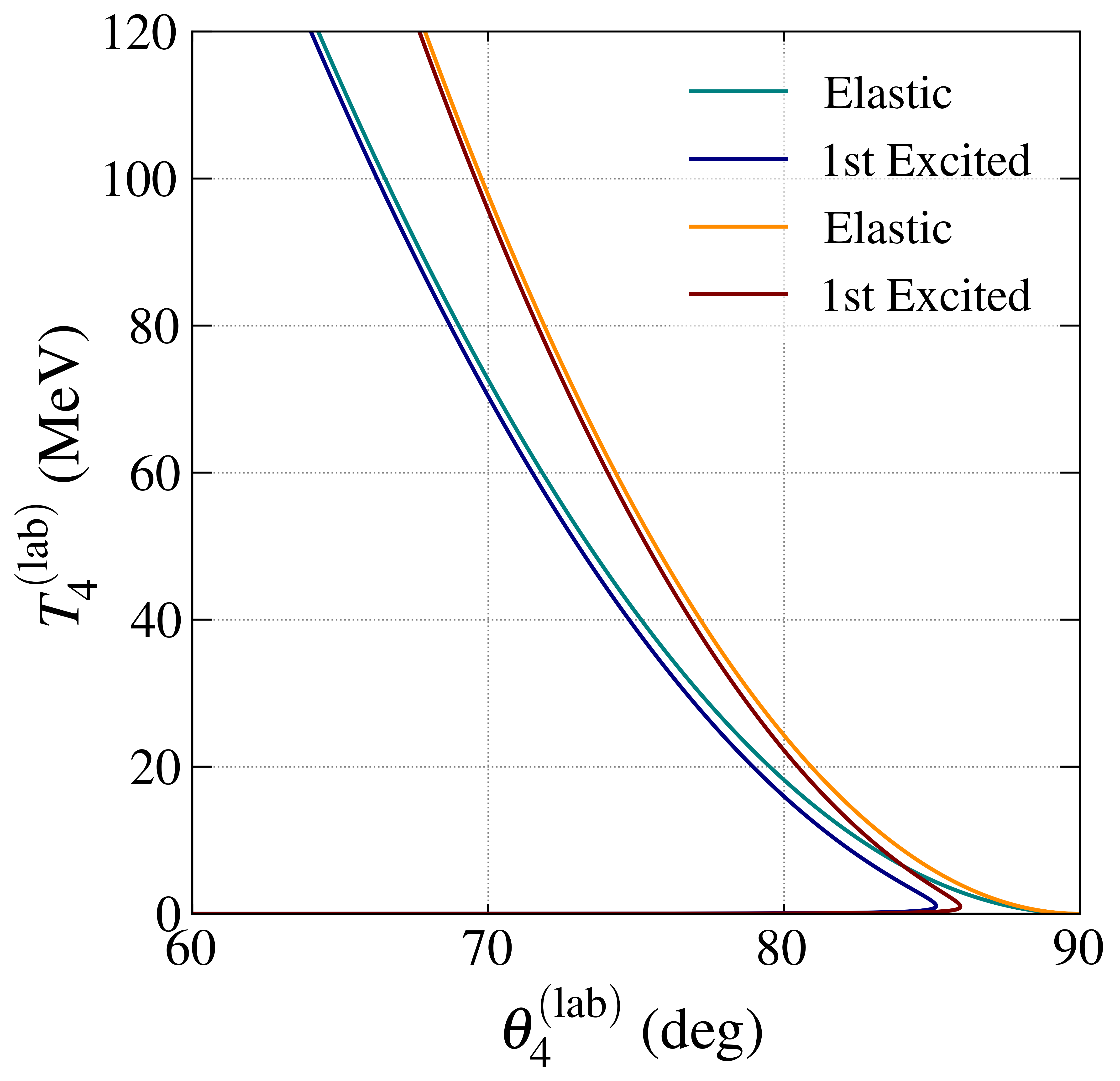
The example below plots the recoil proton's kinetic energy against its lab-frame angle for p(136 Xe, 136 Xe)p at beam energies of 200 and 300 MeV/u.
It also includes the kinematics for excitation of the first excited state of 136 Xe.
import numpy as np import pandas as pd import matplotlib . pyplot as plt from relkin import kinema u = 931.49410372 mass = ( 938.27208943 , 135.907214484 * u , 135.907214484 * u , 938.27208943 ) xe200 = kinema ( * mass ) xe300 = kinema ( * mass ) mass_ex = ( 938.27208943 , 135.907214484 * u , 135.907214484 * u + 1.313 , 938.27208943 ) xe200_ex = kinema ( * mass_ex ) xe300_ex = kinema ( * mass_ex ) xe200 . calc ( 200 * 136 ) xe300 . calc ( 300 * 136 ) xe200_ex . calc ( 200 * 136 ) xe300_ex . calc ( 300 * 136 ) plt . figure ( 0 , figsize = ( 8 , 8 ) , dpi = 600 ) plt . plot ( np . rad2deg ( xe200 . theta4_lab ) , xe200 . T4_lab , color = "teal" , label = "Elastic" , lw = 2 ) plt . plot ( np . rad2deg ( xe200_ex . theta4_lab ) , xe200_ex . T4_lab , color = "navy" , label = "1st Excited" , lw = 2 ) plt . plot ( np . rad2deg ( xe300 . theta4_lab ) , xe300 . T4_lab , color = "darkorange" , label = "Elastic" , lw = 2 ) plt . plot ( np . rad2deg ( xe300_ex . theta4_lab ) , xe300_ex . T4_lab , color = "maroon" , label = "1st Excited" , lw = 2 ) plt . legend ( ) plt . xlim ( 60 , 90 ) plt . ylim ( 0 , 120 )
Cluster Knockout Reaction
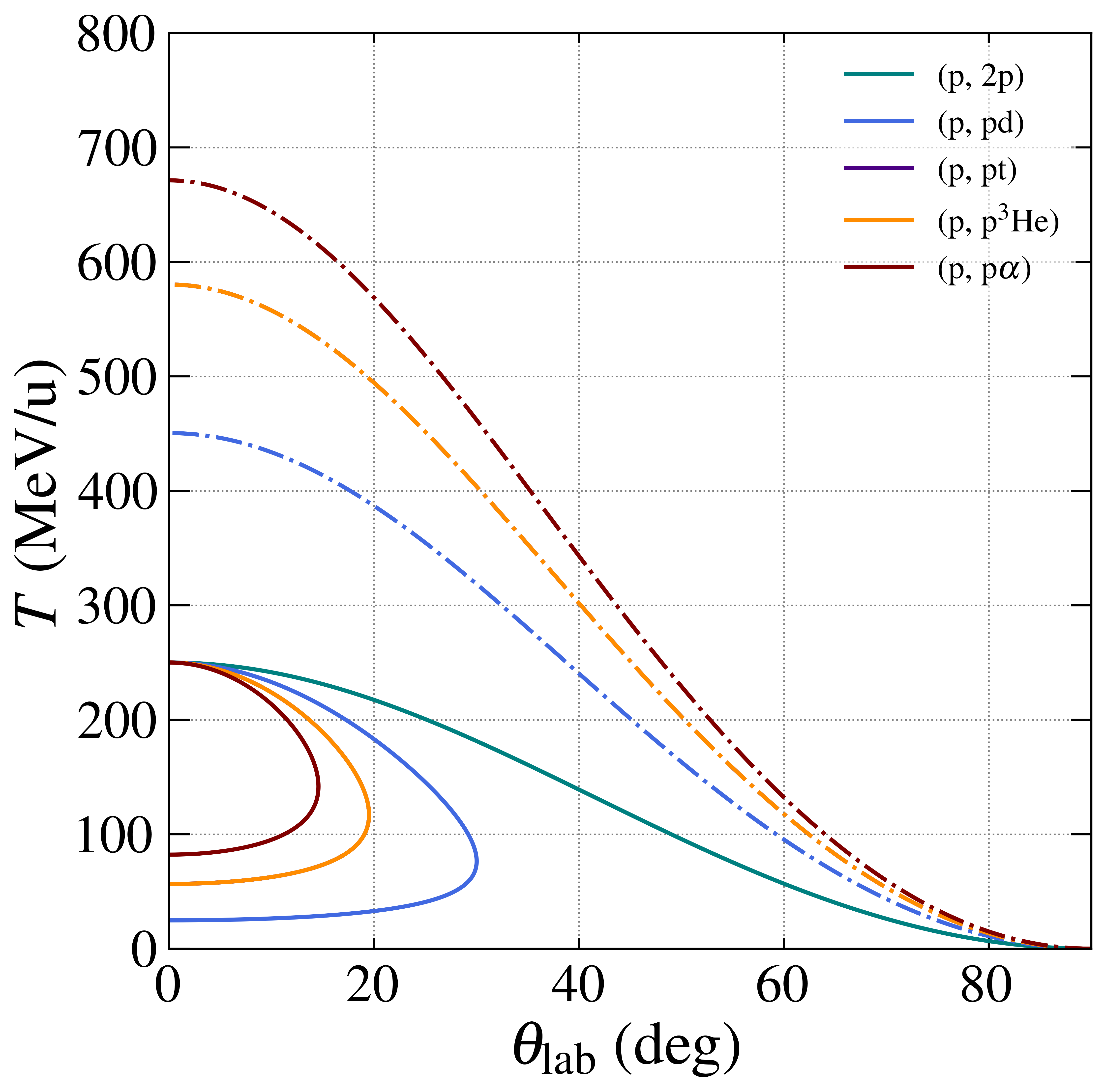
This example plots the kinematics of elastic scattering of p, d, t, 3 He, and α \alpha α
import numpy as np import pandas as pd import matplotlib . pyplot as plt from relkin import kinema u = 931.49410372 mp = 1.00782503223 * u md = 2.01410177812 * u mt = 3.01604927790 * u m3He = 3.01602932007 * u ma = 4.001506179127 * u m_p2p = ( mp , mp , mp , mp ) m_ppd = ( mp , md , md , mp ) m_ppt = ( mp , mt , mt , mp ) m_pp3He = ( mp , m3He , m3He , mp ) m_ppa = ( mp , ma , ma , mp ) kinema_p2p = kinema ( * m_p2p ) kinema_ppd = kinema ( * m_ppd ) kinema_ppt = kinema ( * m_ppt ) kinema_pp3He = kinema ( * m_pp3He ) kinema_ppa = kinema ( * m_ppa ) kinema_p2p . calc ( 250 ) kinema_ppd . calc ( 250 * 2 ) kinema_ppt . calc ( 250 * 3 ) kinema_pp3He . calc ( 250 * 3 ) kinema_ppa . calc ( 250 * 4 ) plt . figure ( 0 , figsize = ( 8 , 8 ) , dpi = 600 ) plt . plot ( np . rad2deg ( kinema_p2p . theta4_lab ) , kinema_p2p . T4_lab / 1 , color = "teal" , label = r"(p, 2p)" , lw = 2 ) plt . plot ( np . rad2deg ( kinema_ppd . theta3_lab ) , kinema_ppd . T3_lab / 2 , color = "royalblue" , label = r"(p, pd)" , lw = 2 ) plt . plot ( np . rad2deg ( kinema_ppd . theta4_lab ) , kinema_ppd . T4_lab , color = "royalblue" , ls = '-.' , lw = 2 ) plt . plot ( np . rad2deg ( kinema_ppt . theta3_lab ) , kinema_ppt . T3_lab / 3 , color = "indigo" , label = r"(p, pt)" , lw = 2 ) plt . plot ( np . rad2deg ( kinema_ppt . theta4_lab ) , kinema_ppt . T4_lab , color = "indigo" , ls = '-.' , lw = 2 ) plt . plot ( np . rad2deg ( kinema_pp3He . theta3_lab ) , kinema_pp3He . T3_lab / 3 , color = "darkorange" , label = r"(p, p$^{3}$He)" , lw = 2 ) plt . plot ( np . rad2deg ( kinema_ppt . theta4_lab ) , kinema_ppt . T4_lab , color = "darkorange" , ls = '-.' , lw = 2 ) plt . plot ( np . rad2deg ( kinema_ppa . theta3_lab ) , kinema_ppa . T3_lab / 4 , color = "maroon" , label = r"(p, p$\alpha$)" , lw = 2 ) plt . plot ( np . rad2deg ( kinema_ppa . theta4_lab ) , kinema_ppa . T4_lab , color = "maroon" , ls = '-.' , lw = 2 ) plt . legend ( ) plt . xlabel ( r"$\theta_\mathrm{lab}$ (deg)" ) plt . ylabel ( r"$T$ (MeV/u)" ) plt . xlim ( 0 , 90 ) plt . ylim ( 0 , 800 )
References